I’m Hydrodynamically Designed!
Why?
Over the last semester, (the fall of 2021 for you historians), I took a class called “Computational Fluid Mechanics and Heat Transfer”. Our professor, Dr. Hanif Montazeri, promised a challenging/rewarding experience; frankly, he undersold it. Over the course of 4 months, we hand-crafted our own solvers for the famous Navier-Stokes Equations. I learned a lot about vector-calculus, discretizing equations, and good programming practice, but most importantly, I made some pretty graphs.
Solvers Specifics
The solver I wrote for this class was written in Python and made extensive use of the SciPy sparse linear algebra library. I used the SIMPLE (Semi-Implicit Method for Pressure Linked Equations) algorithm on a co-located grid. This algorithm was first proposed by Patankar and Spalding in 1973 [1] and its implementation on a co-located grid was first described by Rhie and Chow in 1983 [2]. I promise the pretty graphs are coming.
The Principle Problem
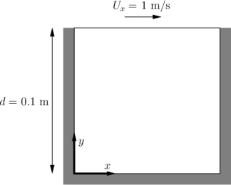
The scope of the course was to simulate the famous “Lid-Driven Cavity” flow problem. This is a well-known benchmark for testing fluid simulations and has been studied numerically and experimentally for decades. The idea is to simulate how a fluid would behave in a square box with an open top where fluid was rushing past:
Ghia et al. [3] wrote a landmark paper in 1982 studying the problem on a high resolution grid. I used their results to verify the correctness of my own solver, which are the first pretty plots I present below:
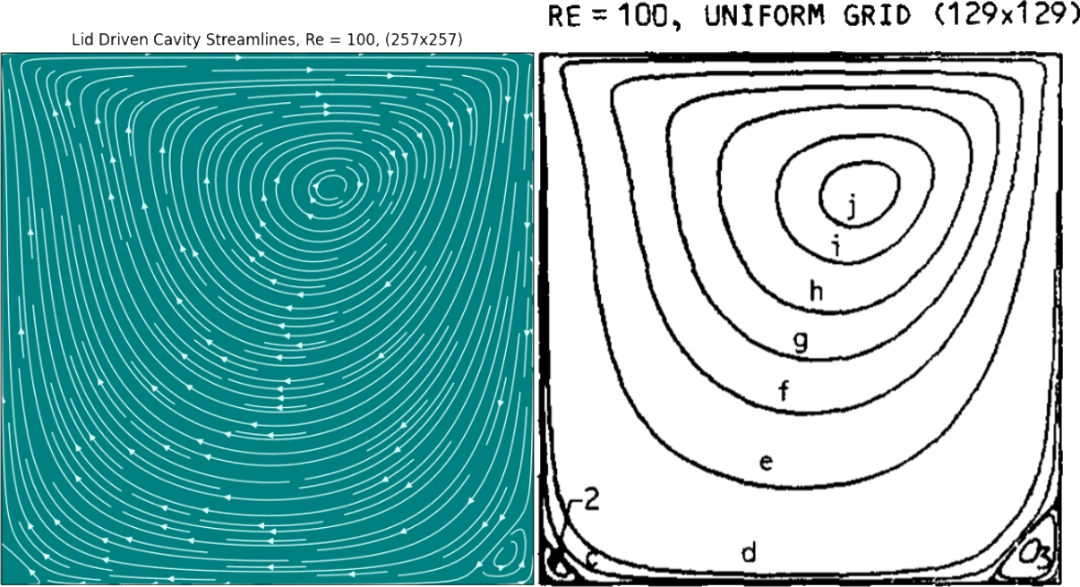
My solver seemed to be accurate enough and I was happy that it captured the small eddies forming in the corners. I also conducted a more involved grid independence study and I compared the velocity profiles through the geometric center of the cavity. These graphs are much less interesting, so for now I hope my readers can take my word for it.
More Interesting Problems
The real beauty of having a solver is that you can go beyond the state-mandated solutions. While developing my code, I made sure to keep it general. There are five specific ways that it is generalized:
- The number of nodes/cells in the domain can be changed
- The aspect ratio of the domain can be changed.
- The velocity at the four boundaries can be changed.
- The Reynolds number can be changed.
- The velocity at any node can be fixed to any value.
Below I present some plots to demonstrate the power of this generalization where possible.
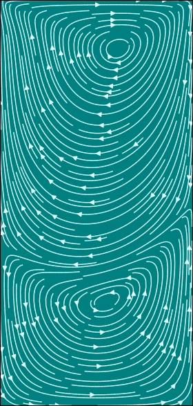
Changing the Aspect Ratio (Point 2)
Flow in a square is cool and all, but variety is the spice of life. How about some rectangles? Below I present the same lid-driven flow problem with differently shaped cavities:
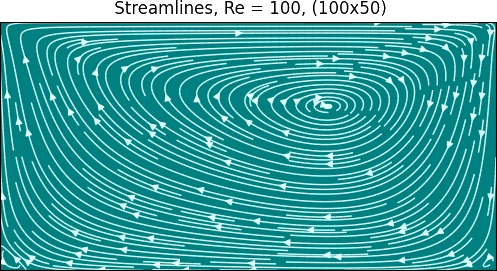
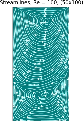
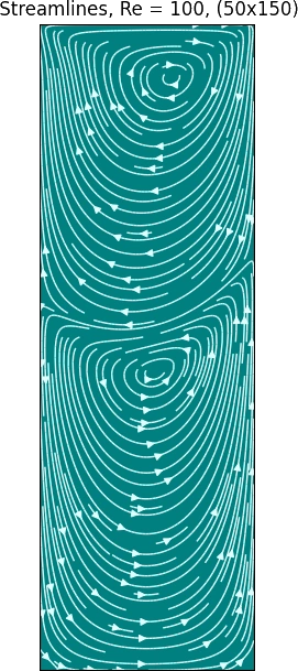
I found the taller boxes more pleasing to look at. Why not make one in the aspect ratio of a phone as a wallpaper? (For Galaxy S10e owners anyway)
Changing the Boundary Conditions (Point 3)
Let’s move beyond your average every day lid driven flow, into advanced lid driven flow. How about a container where the flow on the right and left walls is driven upwards?
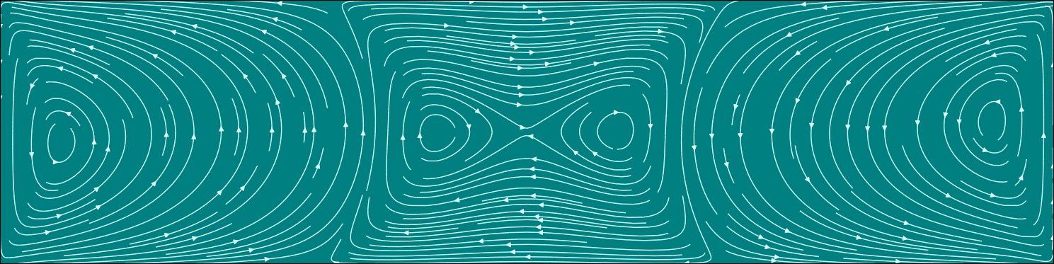
I affectionately refer to this as ‘bowtie flow’
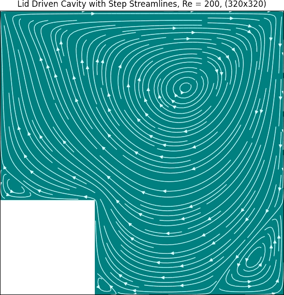
Changing the shape of the domain (Point 5)
Point 5 is especially powerful; it allows us to effectively model flow in or around any shapes. Consider a box with a step in the lower left corner. Simply enough, we can model this by simulating the entire encaspsulating square, and freezing the fluids velocity to zero in places we want to exclude from our domain of interest:
Flow around obstacles (Point 5)
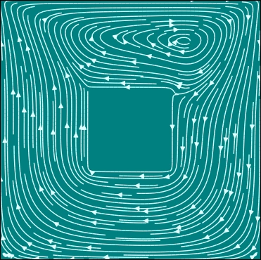
The really fun part about Point 5 is that we can model flow around any arbitray obstacle as well! Below I place a square in the middle of the original lid-driven cavity flow problem:
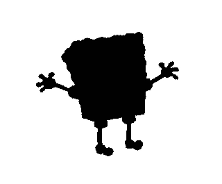
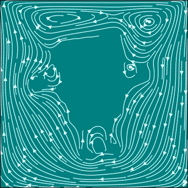
I extended my code so I could take any black and white image and use it as a “mask” to create flow around it as an obstacle. Lets see if old spongebob is as hydrodynamic as he claims. First we start with a profile of our character:

Then we use our editting software of choice to convert this to a black and white mask:
And we plug and play:
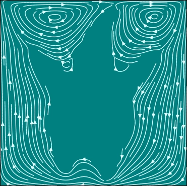
Can you guess this other bikini bottom resident below? Try saving the image for a hint 😉.
Closing thoughts
This project was a ton of fun to work on. I hope to eventually release this code as a webapp or command line app so users can create their own pretty streamlines. There’s a lot more functionality I can see myself adding in the future, including but not limited to:
- Animating flow over moving obstacles
- Pressure boundary conditions
- Symmetry boundary conditions
- Periodic boundary conditions
References
[1] S. V. Patankar and D. B. Spalding, “A calculation procedure for heat, mass and momentum transfer in three-dimensional parabolic flows,” International Journal of Heat and Mass Transfer, vol. 15, no. 10, pp. 1787–1806, Oct. 1972, doi: 10.1016/0017-9310(72)90054-3.
[2] C. M. Rhie and W. L. Chow, “Numerical study of the turbulent flow past an airfoil with trailing edge separation,” AIAA Journal, vol. 21, no. 11, pp. 1525–1532, Nov. 1983, doi: 10.2514/3.8284.
[3] U. Ghia, K. N. Ghia, and C. T. Shin, “High-Re solutions for incompressible flow using the Navier-Stokes equations and a multigrid method,” Journal of Computational Physics, vol. 48, no. 3, pp. 387–411, Dec. 1982, doi: 10.1016/0021-9991(82)90058-4.